Introduction
Data often has an underlying structure or geometry that can be modeled as a signal on the vertices of a weighted, undirected graph. There are several analogies between traditional signal processing and algebraic graph theory that translates many of the tools of discrete signal processing such as spectral analysis of multichannel signals, system transfer function, digital filter design, parameter estimation, and optimal denoising. Historically, graph signal processing (GSP) has focused on modeling smooth signals on a graph, but the increase in availabilty of abstract data sets has led to progress in learning a valid graph given a set of signals.
Preliminaries
A weighted, undirected graph is a triple \(G = (V, E, \omega)\) of two sets \(V = \{1, \ldots, |V| = N \}\) and \(E \subset V \times V\) and a weighting function \(\omega(i,j) = \omega_{i,j}\) that assigns a nonnegative real number to each edge. We can represent a graph by its adjacency matrix \(A\) where \(A_{i,j} = \omega_{i,j}\) if \((i,j) \in E\) and \(0\) otherwise. A signal on a graph \(G\) is a function \(f: V \rightarrow \mathbb{R}\) that can be represented as vector \(x \in \mathbb{R}^N\). The Laplacian of a graph is the matrix \(L = D - A\) where \(D\) is the degree matrix. The Laplacian acts as a difference operator on signals via it’s quadratic form
\[\begin{equation} x^TLx = \sum_{(i,j)\in E}A_{i,j}(x_j - x_i)^2 \end{equation}\]
The Laplacian is positive semi definite, so it has a complete set of orthornormal eigenvectors, and real non negative eigenvalues. Thus, we can diagonalize \(L = \chi^T\Lambda \chi\) where \(\Lambda\) is the diagonal matirx of eigenvalues and \(\chi\) is associated matrix of eigenvectors.
Note that the quadratic form above is minimized when adjacent vertices have identical signal values. This makes program well suited for measuring the smoothness of a signal on a graph. We can cast the problem of learning a graph by the optimization problem found in Kalofolias (2016)
\[\begin{equation} \begin{aligned} \min_L & \phantom{..} \text{tr}(Y^TLY) + f(L),\\ \textrm{s.t.}& \quad \text{tr}(L) = N,\\ & \quad L_{i,j} = L_{j,i} \leq 0, \phantom{..} i \neq j, \\ & \quad L\cdot \textbf{1} = \textbf{0} \end{aligned} \end{equation}\]
Graph Learning Model
Dong et al. propose a modified Factor Analysis model in Dong et al. (2016) for learning a valid graph laplacian. The model proposed is given by \[x = \chi h + \mu_x + \epsilon\] where \(h \in \mathbb{R}^N\) is the latent variable, \(\mu_x \in \mathbb{R}^N\) mean of \(x\). The noise term \(\epsilon\) is assumed to follow a multivariate Gaussian distribution with mean zero and covariance \(\sigma_\epsilon^2I_N\). The key difference from traditional factor analysis is the choice of \(\chi\) as a valid eigenvector matrix for a graph laplacian. Finding a maximum apriori estimate of \(h\) reduces to solving the optimization problem
\[\begin{equation} \begin{aligned} \min_{L \in \mathbb{R}^{N\times N}, \phantom{..} Y \in \mathbb{R}^{N\times P}} ||X&-Y||_F^2 + \alpha \text{tr}(Y^TLY) + \beta||L||_F^2 \\ \textrm{s.t.}& \quad \text{tr}(L) = N, \\ &\quad L_{i,j} = L_{j,i} \leq 0, \phantom{..} i \neq j, \\ &\quad L\cdot \textbf{1} = \textbf{0} \\ \end{aligned} \end{equation}\]
Because the program above is not jointly convex, Dong et al. employ an alternating minimization scheme to solve the problem. Initially, set \(Y = X\) and we find a suitable \(L\) by solving \[\begin{equation} \begin{aligned} \min_L & \phantom{..} \alpha \text{tr}(Y^TLY) + \beta ||L||_F^2, \\ \textrm{s.t.}& \quad \text{tr}(L) = N,\\ & \quad L_{i,j} = L_{j,i} \leq 0, \phantom{..} i \neq j, \\ & \quad L\cdot \textbf{1} = \textbf{0} \end{aligned} \end{equation}\]
Next, using \(L\) from the first step we solve \[\begin{equation} \begin{aligned} \min_Y \phantom{..} ||X-Y||_F^2 + \alpha \text{tr}(Y^TLY) \end{aligned} \end{equation}\]
Both steps can be cast as convex optimazation problems. Specifically, the first problem can be solved with the method of alternating direction of multipliers (ADMM). The second can be solved algebraically. The model is applied to both synthetic and real world data, and compared to a technique used in machine learning that is similar to sparse inverse covariance estimation of Gaussian Markov Random Field models.
Python Implementation
The program of Dong et. al. was originally implemented in MATLAB, but can be solved efficently using the free Python package CVXPY (found here). An implementation of the algorithm can be found here.
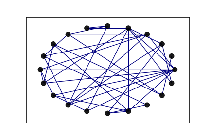
Figure 1: An Erdos-Reyni Graph on 20 nodes, with edge probability 0.2. The ground truth network used to generate 100 synthetic gaussian signals for testing.
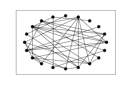
Figure 2: The estimated network. Notice the networks share many features.
This graph was learned with no parameter optimization, but we can see on inspection they share several edges in common. Also, they have the same maximum and minimum degree (8 and 1) and the same total number of edges, \(n = 38\). Detailed results on the preformance of the algrithm with optimized parameters can be found in Dong et al. (2016) .
Contact Info
- GitHub
- Email: skipmoses@gmail.com
Dong, Xiaowen, Dorina Thanou, Pascal Frossard, and Pierre Vandergheynst. 2016. “Learning Laplacian Matrix in Smooth Graph Signal Representations.” IEEE Transactions on Signal Processing 64 (23): 6160–73.
Kalofolias, Vassilis. 2016. “How to Learn a Graph from Smooth Signals.” In Artificial Intelligence and Statistics, 920–29. PMLR.